Axiomatic Approach To Probability

Until now, what we have been doing is simple: to evaluate the probability of any event E in a sample space S, we find the total number of outcomes, and the number of outcomes favorable to E, and we then have

\[P\left( E \right)=\frac{n\left( E \right)}{n\left( S \right)} \qquad\qquad....... (1)\]

You must not at all forget that this holds only if all the outcomes are equally likely, that is, we have no reason to suspect that any particular outcome will be more or less likely than another. For example, we saw that the sample space of tossing a fair coin or rolling a fair die consist of equally likely outcomes. (Note that two outcomes cannot be proved mathematically to be equally likely. We either assume beforehand the equal likelihood of outcomes, or we repeat the experiment an indefinitely large number of times, and thus show empirically (rather than mathematically) that the relative frequencies of the various outcomes approach the same value).

Now, coming back to (1), we said that it will not hold if the various outcomes are not equally likely. For example, suppose that a die is constructed (using careful loading) such that

\[P\left( 1 \right)=P\left( 2 \right)=P\left( 3 \right)=\frac{1}{6},\,P\left( 4 \right)=\frac{1}{3},\,P\left( 5 \right)=\left( \frac{1}{8} \right),\,\,P\left( 6 \right)=\frac{1}{24}\]

For such a die, the probability of rolling an odd number will be

\[P\left( 1 \right)=P\left( 3 \right)=P\left( 5 \right)=\frac{1}{6}+\frac{1}{6}+\frac{1}{8}=\frac{11}{24}\]

rather than \(\begin{align}\frac{1}{2}\end{align}\) , which you would have got by doing (no. of odd outcomes / no. of total outcomes). This point is easy to understand yet mistakes are made!

A curious reader might have a further issue. She might say, “You just talked about making a die with outcomes of unequal probabilities. For example, you said that \(\begin{align}P\left( 5 \right)=\frac{1}{8}.\end{align}\) What is the basis for saying so? I understood the case of equally likely outcomes, where all probabilities are the same, but how did this figure of \(\begin{align}\frac{1}{8}\end{align}\) come about ?” Well, this number comes about by using a relative frequency approach to probability. When the die-maker says that the probability of a 5 coming up is \(\begin{align}\frac{1}{8}\end{align}\) , what he must have done (either actually, or through a sophisticated computer simulation) is roll the die a very large number of times, and observe that 5 comes up (about) one-eight of the time. Thus the assertion.

To summarize, there are two ways we’ve discussed to evaluate probabilities

* Classical approach : this ‘works’ when all the outcomes are equally likely. If our event can happen in n ways out of a total possible of N, our required probability is n/N

* Frequency approach : this ‘works’ in general. To find the probability of an event, we repeat the experiment a very large number of times, say M, and observe how many times that particular event occurred, say m. m/M then gives us the empirical probability of an event. In fact, we should be using this relation:

\[P\left( \text{event} \right)=\underset{M\to \infty }{\mathop{\lim }}\,\frac{m}{M}\]

that is, we should be using the value of empirical probability only if the experiment is repeated an indefinitely large number of times.

Finally, it must be said that both the approaches fail to stand up to the rigors of mathematics, because the former uses the vague phrase “equally likely” about which we can give no mathematical justification, while in the latter, we have no way to prove that the limit \(\begin{align}\underset{M\to  \infty }{\mathop{\lim }}\,\frac{m}{M}\end{align}\) will actually coverage to some value, because no experiment can be repeated an infinite number of times.

Mathematicians therefore, being very finicky about rigor, define probability as a function associated with any event and that satisfies three axioms:

Axiom 1 : For any event E,

\[0\le P\left( E \right)\le 1\]

Axiom 2 : For the entire sample space S (that is, for the sure event),

\[P\left( S \right)=1\]

Axiom 3 : For mutually exclusive events \({{A}_{i}},\,\,i=1,\,\,2,...,\)

\[P\left( {{A}_{1}}\cup {{A}_{2}}\cup ... \right)=P\left( {{A}_{1}} \right)+P\left( {{A}_{2}} \right)+....\]

Thus, what we have here is three axioms that the probability of any event(s) must satisfy, but these three axioms in no way tell us how to actually measure probability associated with any event. Those interested in knowing more deeply about these axioms and the interpretation of probability should find plenty of resources on the World Wide Web. For present, this much background should suffice.

Before closing this section, let us see some more examples of how events are treated as subsets of a universal set of outcomes, the sample space. Events are denoted by A, B, C etc and the sample space by S. The complementary event of any event A is denoted by \(\bar{A}\) .

Relation	Venn diagram
(1) \(P\left( A \right)+P\left( {\bar{A}} \right)=P\left( S \right)=1\)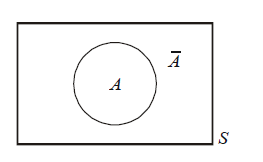
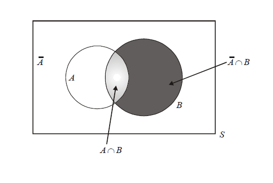
(2) \(P\left( A\cap \bar{B} \right)=P\left( A \right)-P\left( A\cap B \right)\)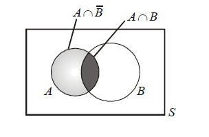
(3) \(P\left( A\cup B \right)=P\left( A \right)+P\left( B \right)-P\left( A\cap B \right)\)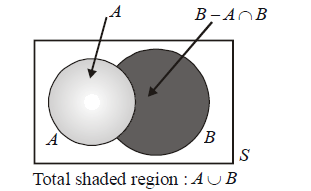

Generalising this gives

\[\begin{align} & P\left( {{A}_{1}}\cup {{A}_{2}}\cup ...\cup {{A}_{n}} \right)=\sum\limits_{i=1}^{n}{P\left( {{A}_{i}} \right)}-\sum\limits_{i<j}^{{}}{P\left( {{A}_{i}}\cap {{A}_{j}} \right)}+\sum\limits_{i<j<k}^{{}}{P\left( {{A}_{i}}\cap {{A}_{j}}\cap {{A}_{k}} \right)} \\  &\qquad\qquad\qquad\qquad\qquad\qquad -...+{{\left( -1 \right)}^{n-1}}P\left( {{A}_{1}}\cap {{A}_{2}}...\cap {{A}_{n}} \right) \\ \end{align}\]

For example,

\[\begin{align}& P\left( {{A}_{1}}\cup {{A}_{2}}\cup {{A}_{3}} \right)=P\left( {{A}_{1}} \right)+P\left( {{A}_{2}} \right)+P\left( {{A}_{3}} \right)-P\left( {{A}_{1}}\cap {{A}_{2}} \right)-P\left( {{A}_{2}}\cap {{A}_{3}} \right) \\ &\qquad\qquad\qquad\qquad -P\left( {{A}_{3}}\cap {{A}_{1}} \right)+P\left( {{A}_{1}}\cap {{A}_{2}}\cap {{A}_{3}} \right) \\ \end{align}\]

Try proving this relation for three events using a Venn diagram

(4)   \(P\left( {{A}_{1}}\cup {{A}_{2}} \right)\le P\left( {{A}_{1}} \right)+P\left( {{A}_{2}} \right)\)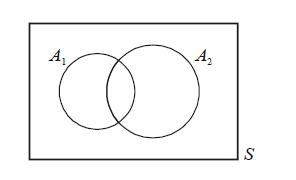

This should be obvious. On the right side of the inequality, there is an extra contribution to the sum from  \({{A}_{1}}\cap {{A}_{2}}.\) The equality holds only for mutually exclussive events.

This also generalises obviously to n events.

(5)  \(P\left( {{{\bar{A}}}_{1}} \right)+P\left( {{{\bar{A}}}_{2}} \right)\ge 1-P\left( {{A}_{1}}\cap {{A}_{2}} \right)\)

Try to figure this out on your own. Using a Venn diagram would be a good idea.

Example – 11

For two events A and B, find the probability that exactly one of the two events occur.

Solution: This can happen in two ways:

Way                                                        Set of outcomes

A occurs, B doesn’t                       :                 \(A\cap \bar{B}\)               B occurs, A doesn’t                       :                    \(\bar{A}\cap B\)

 

Note that the two ways are ME. Thus, the required probability is \(P\left( A\cap \bar{B} \right)+P\left( \bar{A}\cap B \right)\)  , which from the second relation becomes

\[P\left( A \right)\text{ }P\left( A\cap B \right)+P(B)-P\left( A\cap B \right)=P\left( A \right)+P(B)-2P\left( A\cap B \right)\]

Justify this last expression using a Venn diagram, by shading the area it represents.

Example – 12

For two events A and B, show that

\[P\left( B \right)=P\left( A \right)\cdot P\left( B/A \right)+P\left( {\bar{A}} \right)\cdot P\left( B/\bar{A} \right)\]

Solution: This is straightforward, since

\[P\left( A \right)\cdot P\left( B/A \right)=P\left( A\cap B \right)\,\,\,\,\,\,\,\,\,\,\,\,\,\,\,\,\,\,\,\,\,\left\{ \begin{align}& \text{recall the discuss in} \\ & \text{the previous section} \\ \end{align} \right\}\]

and

\[P\left( {\bar{A}} \right)\cdot P\left( B/\bar{A} \right)=P\left( \bar{A}\cap B \right)\]

Now, since \(A\,\,\text{and}\,\,\bar{A}\) are mutually exclusive, we must have

\[P\left( A\cap B \right)+P\left( \bar{A}\cap B \right)=P\left( B \right)\]

TRY YOURSELF - II

Q. 1 For three events A, B, C, show that

(a) P (at least two of A, B, C occur) =

\[P\left( A\cap B \right)+P\left( B\cap C \right)+P\left( C\cap A \right)-2P\left( A\cap B\cap C \right)\]

(b) P (exactly two of A, B, C occur) =

\[P\left( A\cap B \right)+P\left( B\cap C \right)+P\left( C\cap A \right)-3P\left( A\cap B\cap C \right)\]

(c) P (exactly one of A, B, C occurs) =

\[P\left( A \right)+P\left( B \right)+P\left( C \right)-2P\left( A\cap B \right)-2P\left( B\cap C \right)-2P\left( C\cap A \right)+3P\left( A\cap B\cap C \right)\]