Newton Leibnitz Formula

Our approach in this section will be to lay the groundwork on which all the tools and techniques of integration will be built in the coming sections. Let us take an arbitrary curve \(y = f\left( x \right).\) Our purpose is to find the area under this curve from \(x = a \;\; to \;\; x = b.\)

What we first do is fix an arbitrary point on the number line, say x = 0, and let our variable x move on the number line.

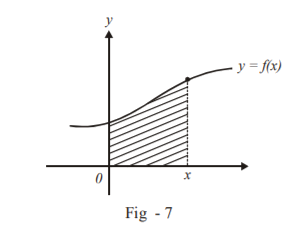
The area under the curve \(y = f\left( x \right)\) from 0 to x will obviously be some function of x. Let us denote this function by \({\rm{g(x) : g(x)}}\) denotes the area under \(y = f\left( x \right)\) from 0 to x.

\[g\left( x \right) = \int\limits_0^x {f\left( x \right)dx} \]

To avoid confusion, we can denote the integration variable (the variable that goes from 0 to x) by x' instead of x, so that:

     \[g\left( x \right) = \int\limits_0^x {f\left( {x'} \right)dx'} \]

Now let us evaluate the derivative of g(x) at an arbitrary x:

\[\begin{align}&\frac{{d\left( {g\left( x \right)} \right)}}{{dx}} = \mathop {\lim }\limits_{h \to 0} \frac{{g\left( {x + h} \right) - g\left( x \right)}}{h}\\ &\qquad\qquad= \mathop {\lim }\limits_{h \to 0} \left\{ {\frac{{\int\limits_0^{x + h} {f\left( {x'} \right)dx' - \int\limits_0^x {f\left( {x'} \right)dx'} } }}{h}} \right\}\end{align}\]

Notice that in the expression above, the numerator represents the difference in area under the curve from \((0\; to\; x + h) \) from the area under the curve from (0 to x); what should be the result: the area under the curve from x to x + h.

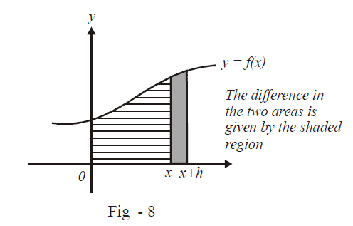
Therefore,

\[\frac{{d\left( {g\left( x \right)} \right)}}{{dx}} = \mathop {\lim }\limits_{h \to 0} \left\{ {\frac{{\int\limits_x^{x + h} {f\left( {x'} \right)dx'} }}{h}} \right\}\]

Now think about the right hand side expression carefully. The numerator represents the area under the curve from x to x + h. h is an infinitesimally small quantity.

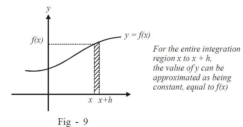
Therefore, in the integration region x to x + h, we can approximate the function’s value as f(x) itself, because in such a small interval, the variation in f(x) is also infinitesimally small. Hence, we can approximate this infinitesimally small area as a rectangle of width h and height f(x); you must convince yourself that as \(h \to 0,\) this approximation becomes more and more accurate. Now using this argument further, we get:

\[\begin{align}&\frac{{d\left( {g\left( x \right)} \right)}}{{dx}} = \frac{{f\left( x \right) \times h}}{h}\\ &\qquad\qquad= f\left( x \right)!\end{align}\]

This simple result shows that the function g(x) is simply such that its derivative equals f(x). g(x) is termed the anti-derivative of f(x); the name is self-explanatory.

For example, the anti derivative of \(f\left( x \right) = {x^2}\) would be \(\begin{align}&g\left( x \right) = \frac{{{x^3}}}{3} + c\end{align}\) (c is a constant so its inclusion in the expression of g(x) is valid as  \(\begin{align}&\frac{{d\left( c \right)}}{{dx}} = 0)\end{align}\):

\[\begin{align}&\frac{{d\left( {g\left( x \right)} \right)}}{x} = \frac{d}{{dx}}\left( {\frac{{{x^3}}}{3} + c} \right)\\ &\qquad\qquad= \frac{{3{x^2}}}{3} + 0\\ &\qquad\qquad= {x^2}\end{align}\]

Similarly, the anti derivative of f(x) = cos x would be g(x) = sin x + c since

\[\frac{{d\left( {g\left( x \right)} \right)}}{{dx}} = \frac{{d\left( {\sin x + c} \right)}}{{dx}}\\\;\;= \cos x\]

Now, returning to our original requirement, how do we find out the area under f(x) using the anti-derivative; this is now quite straight forward. Suppose our requirement is to find the area under the curve f(x) from x = a to x = b.

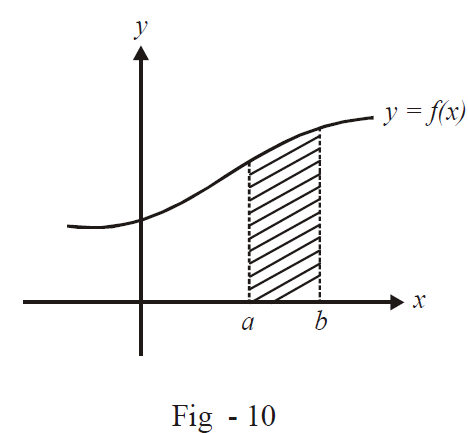
We can equivalently evaluate this area by calculating the area from 0 to b and subtracting from it the area under the curve from 0 to a:

\[\int\limits_a^b {f\left( x \right)dx = \int\limits_0^b {f\left( x \right)dx--\int\limits_0^a {f\left( x \right)dx} } } \]

But we just defined the anti derivative as

\[g\left( x \right) = \int\limits_0^x {f\left( {x'} \right)dx'} \]

Therefore,

 \[\begin{array}{l}\int\limits_0^b {f\left( x \right)dx = g\left( b \right)} \\\int\limits_0^a {f\left( x \right)dx = g\left( a \right)} \end{array}\]

and the required area under the curve simply becomes

\[\boxed{\int\limits_a^b {f\left( x \right)dx = g\left( b \right) - g\left( a \right)}}\]

This extraordinary result is the Newton Leibnitz formula. What it says is that to evaluate the area under f(x) from a to b, evaluate the anti derivative g(x) of f(x) and then find \(g\left( b \right)-g\left( a \right).\)

(Note that there is nothing special about the lower limit in the anti-derivative integral being 0; it could have been any arbitrary constant, the final outcome is not in anyway related to this constant; it was just selected as a reference point).

You must ensure, for a good understanding of calculus, that you’ve entirely followed this discussion; if not, you must re-read it till you fully understand it.

The next chapter is entirely devoted to developing ways to find out the anti-derivative of an arbitrary given function. The process of finding out the anti-derivative is called indefinite integration; the anti-derivative is also referred to as the indefinite integral. When we actually substitute the limits of integration (the two x-values between which we want to find out the area) into the anti-derivative, i.e., when we calculate \(g\left( b \right)-g\left( a \right)\), the process is known as definite integration. The adjectives indefinite and definite are self-explanatory.

EXERCISE

Q.1  Evaluate the following “definite” integrals by first principles:

(a) \(\int\limits_0^1 {x\,\,\,dx} \)	(b) \(\int\limits_{ - 2}^2 {{x^2}dx} \)
(c) \(\int\limits_0^3 {{x^3}dx} \)	(d)\(\int\limits_{ - 3}^3 {{x^3}dx} \)
(e) \(\int\limits_0^1 {{e^x}dx} \)	(f) \(\int\limits_0^1 {\sqrt x dx} \)
(g) \(\int\limits_{ - 1}^1 {\left( {{x^2} + x + 1} \right)dx} \)	(h) \(\int\limits_{ - 2}^3 {\left[ x \right]dx} \)
(i) \(\int\limits_0^{10} {\left\{ x \right\}dx} \)	(j)\(\int\limits_2^3 {\left| x \right|dx} \)

Q.2  Try to “guess” the anti-derivatives of the following functions:

(a) \(f\left( x \right) = {x^5} + {x^4}\)	(b)\(f\left( x \right) = {\sec ^2}x\)
(c) \(f\left( x \right) = \tan x\)	(d) \(\begin{align}f\left( x \right) = \frac{1}{{1 + {x^2}}}\end{align}\)
(e) \(f\left( x \right) = \sqrt x \)