Six Basic Inverse Trigonometric Functions

Recall the following facts about inverse functions:

• For a function  \(f:A \to B\), we can define  \({f^{ - 1}}\) on this pair of sets  \(A,\;B\)  if f is a bijection, that is, f is one-one and onto
• Given that this constrain is satisfied, we can define  \({f^{ - 1}}\) as  \({f^{ - 1}}:B \to A\)  such that \(f({f^{ - 1}}(x)) = {f^{ - 1}}(f(x)) = x\). For example, for  \(f:\left[ {0,\;\infty } \right) \to \left[ {0,\;\infty } \right)\) given by  \(f(x) = {x^2}\), the inverse function is defined as  \({f^{ - 1}}:\left[ {0,\;\infty } \right) \to \left[ {0,\;\infty } \right)\)  and given by  \({f^{ - 1}}(x) = \sqrt x \).
• The graphs of  \(f(x)\) and  \({f^{ - 1}}(x)\)  are mirror reflections of each other in the line  \(y = x\).

In this section, our purpose is to define the inverses of all the trigonometric functions and understand their behavior and properties. Since all the trigonometric functions are periodic, they are not bijections over their entire domains. The means that we have to restrict the domains of definition of these functions when defining their inverses, so that the functions are bijections over the restricted domains. However, there can be many such restricted domains over which a given trigonometric function is a bijection. Conventionally, we choose one of these to define the inverse.

For example  \(f(x) = \sin x\), is a bijection over both  \(\begin{align}\left[ {\frac{{ - \pi }}{2},\;\frac{\pi }{2}} \right]\;\;{\text{and}}\;\;\left[ {\frac{\pi }{2},\frac{{3\pi }}{2}} \right]\end{align}\), but it is the first interval over which we define the inverse of. You could call it a matter of convention and/or convenience.

Let us define the various trigonometric inverses now.

(1)  \(f(x){\mathbf{ = si}}{{\mathbf{n}}^{{\mathbf{-1}}}}x\)

We restrict the domain of  \(\begin{align}\sin x\;{\text{to}}\;\left[ {\frac{{ - \pi }}{2},\;\frac{\pi }{2}} \right]\end{align}\), since over this interval, is a bijection. Thus, we redefine   \(\sin x\)   as

\[g(x) = \sin x,\;\left[ {\frac{{ - \pi }}{2},\;\frac{\pi }{2}} \right] \to \left[ { - 1,\;1} \right]\]

Thus we have

\[f(x) = {\sin ^{ - 1}}x,\;[ - 1,\;1] \to \left[ {\frac{{ - \pi }}{2},\;\frac{\pi }{2}} \right]\]

To understand the behavior of  \({\sin ^{ - 1}}x\), we flip the graph of (the appropriate segment of)  \(\sin x\) about the line \(y = x:\)

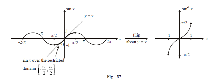
Note the slopes of  \( {\sin ^{ - 1}}x\)  carefully. It is vertical at the points  \(x =  \pm 1\)  and has a slope of 1 at x = 0. Also, it is strictly increasing, since  \(\sin x\) itself is strictly increasing over \(\begin{align}\left[ {\frac{{ - \pi }}{2},\;\frac{\pi }{2}} \right]\end{align}\).

Following this approach, we define the other inverses similarly. The only important thing to keep in mind is that the original function must be restricted to a domain where it becomes a bijection.

 

(2)  \(f(x){\mathbf{ = co}}{{\mathbf{s}}^{{\mathbf{-1}}}}x\)

We define as

\[g(x) = \cos x,\;[0,\;\pi ] \to [-1,\;1]\]

so that

\[f(x) = {\cos ^{ -1}}x,\;[ -1,\;1] \to [0,\;\pi ]\]

Once again, note the slopes of   \({\cos ^{ -1}}x\). It is strictly decreasing since cos x is strictly decreasing.

 

(3) \(f(x) = {\mathbf{ta}}{{\mathbf{n}}^{{\mathbf{-1}}}}x\)

We define as

\[g(x) = \tan x,\;\left( {\frac{{ - \pi }}{2},\;\frac{\pi }{2}} \right) \to \mathbb{R}\]

so that

\[f(x) = {\tan ^{ - 1}}x,  \mathbb{R} \to \left( {\frac{{ - \pi }}{2},\;\frac{\pi }{2}} \right)\]

Note that is strictly increasing. Also, at  \(x = 0,\;\left( {{{\tan }^{ - 1}}x} \right)' = 1\)

 

(4)  \(f(x){\mathbf{ = co}}{{\mathbf{t}}^{{\mathbf{-1}}}}x\)

We define as

\[g(x) = \cot x,\;(0,\;\pi ) \to \mathbb{R}\]

so that

\[f(x) = {\cot ^{ - 1}}x,\;\mathbb{R} \to (0,\;\pi )\]

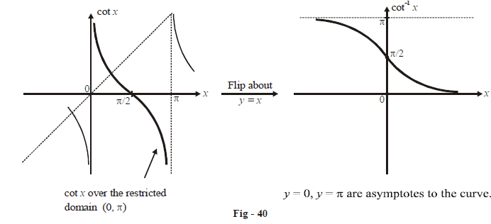
Note that \({\cot ^{ - 1}}x\)  is strictly decreasing, and that  \(({\cot ^{ - 1}}x)'\)  at  \(x = 0\) is –1.

 

(5) \(f(x){\mathbf{ = se}}{{\mathbf{c}}^{{\mathbf{-1}}}}x\)

We define as

\[g(x) = \sec x,\;[0,\;\pi ]\;\backslash \left\{ {\frac{\pi }{2}} \right\} \to \left( { - \infty ,\; - 1} \right] \cup \left[ {1,\;\infty } \right)\]

so that

\[f(x) = {\sec ^{ - 1}}x,\;\left( { - \infty ,\; - 1} \right] \cup \left[ {1,\;\infty } \right) \to [0,\;\pi ]\backslash \left\{ {\pi /2} \right\}\]

Note that  \({\sec ^{ - 1}}x\) is strictly increasing over  \(\left( { - \infty ,\; - 1} \right]\;{\text{and}}\;\left[ {1,\;\infty } \right)\). Also  \(x =  \pm 1\) \(({\sec ^{ - 1}}x)\) at, is infinite, i.e., the curves are ‘vertical’.

 

(6)  \(f(x) = {\text{cose}}{{\text{c}}^{ - 1}}x\)

We define cosec x as

\[g(x) = {\text{cosec}}\,x,\;\left[ {\frac{{ - \pi }}{2},\;\frac{\pi }{2}} \right]\backslash \left\{ 0 \right\} \to [ - \infty ,\; - 1]\; \cup \left[ {1,\;\infty } \right)\]

so that

\[f(x) = {\text{cose}}{{\text{c}}^{ - 1}}\,x,\;\left( { - \infty ,\; - 1} \right]\; \cup \left[ {1,\;\infty } \right) \to \left[ {\frac{{ - \pi }}{2},\;\frac{\pi }{2}} \right]\;\backslash \;\left\{ 0 \right\}\]

\({\text{cose}}{{\text{c}}^{ - 1}}x\)  is strictly decreasing on  \(\left( { - \infty ,\; - 1} \right]\;{\text{and}}\;{\text{on}}\;\left[ {1,\;\infty } \right)\). At \(x =  \pm \;1,\) its slopes are vertical.

From the graphs of the inverse functions, note the following properties:

\[{\sin ^{ - 1}}( - x) =  - {\sin ^{ - 1}}x, \qquad  {\cos ^{ - 1}}( - x) = \pi  - {\cos ^{ - 1}}(x), \qquad {\tan ^{ - 1}}( - x) =  - {\tan ^{ - 1}}x\]

\[{\text{cose}}{{\text{c}}^{ - 1}}( - x) =  - {\text{cose}}{{\text{c}}^{ - 1}}x, \qquad {\sec ^{ - 1}}( - x) = \pi  - {\sec ^{ - 1}}(x), \qquad  {\cot ^{ - 1}}( - x) = \pi  - {\cot ^{ - 1}}x\]

We have seen that  \({f^{ - 1}}(f(x)) = f({f^{ - 1}}(x)) = x\). For example,

\[\begin{align}&\sin \left( {{{\sin }^{ - 1}}\left( {\frac{1}{2}} \right)} \right) = \sin \left( {\frac{\pi }{6}} \right) = \frac{1}{2}  \\  &{\sin ^{ - 1}}\left( {\sin \left( {\frac{\pi }{6}} \right)} \right) = {\sin ^{ - 1}}\left( {\frac{1}{2}} \right) = \frac{\pi }{6}\quad etc. \\ \end{align} \]

But this relation must be used with caution, since it is valid only if x lies in the appropriate domain. For example,

\[{\sin ^{ - 1}}\left( {\sin \left( {\frac{{5\pi }}{6}} \right)} \right) = {\sin ^{ - 1}}\left( {\frac{1}{2}} \right) = \frac{\pi }{6}\;\;{\text{and}}\;{\mathbf{not}}\;\frac{{5\pi }}{6}\]

Therefore \({\sin ^{ - 1}}(\sin \theta )\), will not always be  \(\theta \), since the output of  \({\sin ^{ - 1}}\) will necessarily lie in the range  \(\begin{align}\left[ {\frac{{ - \pi }}{2},\;\frac{\pi }{2}} \right]\end{align}\). To adjust for this fact, note the following:

\[\begin{align}&{\sin ^{ - 1}}(\sin \theta ) = \left\{ \begin{gathered}- \pi  - \theta ,\;\;{\text{if}}\;\theta  \in \;\left[ {\frac{{ - 3\pi }}{2},\;\frac{{ - \pi }}{2}} \right] \\  \;\;\;\;\;\theta ,\;\;\;\;{\text{if}}\;\theta  \in \;\left[ {\frac{{ - \pi }}{2},\;\frac{\pi }{2}} \right]  \\  \pi  - \theta ,\;\;\;\;{\text{if}}\;\theta  \in \;\left[ {\frac{\pi }{2},\;\frac{{3\pi }}{2}} \right]  \\   - 2\pi  + \theta ,\mathop {{\text{if}}}\limits_ \vdots  \;\theta  \in \;3\pi /2,\;5\pi /2   \\ \end{gathered}  \right\} \qquad\left({{\text{Verify!}}} \right)  \\  &\qquad\qquad\qquad\qquad\qquad{\text{and}}\;{\text{so}}\;{\text{on}} \\ \end{align} \]

That is, we have adjusted the output values so that they always fall within the interval  \(\begin{align}\left[ {\frac{{ - \pi }}{2},\;\frac{\pi }{2}} \right]\end{align}\). Here’s the graph of  \({\sin ^{ - 1}}(\sin \theta )\). Make sure you understand it properly:

So, no matter what the value of  \(\theta \), the output of  \({\sin ^{ - 1}}(\sin \theta )\)  will always fall in the range \(\begin{align}\left[ {\frac{{ - \pi }}{2},\;\frac{\pi }{2}} \right]\end{align}\).

Similarly, we have

\[\begin{align}&\;\;\;\;\;\;\;\;\;\;\;\;\;\;\;\;\;\;\;\;\;\;\;\;\;\;\;\;\;\;\;\;\;\;\;\;\;\;\; \vdots  \\ & {\cos ^{ - 1}}(\cos \theta ) = \left\{ \begin{gathered}  \; - \theta \;,\;\;\;\;\;\;\;\;\;{\text{if}}\;\theta  \in [ - \pi ,0] \\  \;\;\;\theta \;\;\;,\;\;\;\;\;\,{\text{if}}\;\theta  \in [0,\;\pi ]  \\  2\pi  - \theta ,\;\;\;\;\;\;{\text{if}}\,\theta  \in [\pi ,\;2\pi ]\; \\   - 2\pi  + \theta ,\;\;\,\,\,{\text{if}}\;\theta  \in [2\pi ,3\pi ]\; \\ \end{gathered}  \right\} \\&\;\;\;\;\;\;\;\;\;\;\;\;\;\;\;\;\;\;\;\;\;\;\;\;\;\;\;\;\;\;\;\;\;\;\;\;\;\;\; \;\;\; \vdots \\  &\qquad\qquad\qquad\qquad\qquad\;\;{\text{and}}\;{\text{so}}\;{\text{on}}  \\ \end{align} \]

Similarly,

\[\begin{align}&\quad\;\;\;\;\;\;\;\;\;\;\;\;\;\;\;\;\;\;\;\;\;\;\;\;\;\;\;\;\;\;\;\;\;\;\;\;\; \vdots   \\ &{\tan ^{ - 1}}(\tan \theta ) = \left\{ \begin{gathered}  \pi  - \theta ,\;\;{\text{if}}\;\theta  \in \left( {\frac{{ - 3\pi }}{2},\;\frac{{ - \pi }}{2}} \right) \\  \,\,\,\,\theta \,\,\,,\;\;\;{\text{if}}\;\theta  \in \left( {\frac{{ - \pi }}{2},\;\frac{\pi }{2}} \right) \\\theta  - \pi ,\;\;{\text{if}}\;\theta  \in \left( {\frac{\pi }{2},\;\frac{{3\pi }}{2}} \right) \\ \end{gathered}  \right\} \\  &\quad\;\;\;\;\;\;\;\;\;\;\;\;\;\;\;\;\;\;\;\;\;\;\;\;\;\;\;\;\;\;\;\;\;\;\;\;\; \vdots  \\  &\qquad\qquad\qquad\qquad\qquad{\text{and}}\;{\text{so}}\;{\text{on}} \\ \end{align}\]

Plotting the graph of  \({\tan ^{ - 1}}(\tan \theta )\)  is left to the reader as an exercise.

Inverse trigonometric functions satisfy other interesting properties that you must be familiar with. For example, for \(x \in \left( { - \infty ,\; - 1} \right] \cup \left[ {1,\;\infty } \right)\)

\[{\sin ^{ - 1}}\left( {\frac{1}{x}} \right) = {\text{cose}}{{\text{c}}^{ - 1}}x\]

The justification is easy. If  \({\text{cose}}{{\text{c}}^{ - 1}}x = \theta ,\)  then  \(x = {\text{cosec}}\theta ,\)  which means that   \(\begin{align}\frac{1}{x} = \sin \theta,\end{align}\)  so that  \(\begin{align}{\sin ^{ - 1}}\left( {\frac{1}{x}} \right) = \theta  = {\text{cose}}{{\text{c}}^{ - 1}}x\end{align}\).

Similarly, we’ll have

\[{\cos ^{ - 1}}\left( {\frac{1}{x}} \right) = {\sec ^{ - 1}}x,\;{\text{for}}\;x \in \left( { - \infty ,\; - 1} \right] \cup \left[ {1,\;\infty } \right)\]

The relation between  \({\tan ^{ - 1}}\;{\text{and}}\;{\cot ^{ - 1}}\)  is :

\[{\tan ^{ - 1}}\left( {\frac{1}{x}} \right) = \left\{ \begin{align}{\cot ^{ - 1}}x,\;\;\;\;\;\;\;\;x > 0  \\   - \pi  + {\cot ^{ - 1}}x,\;x < 0\\ \end{align}  \right\}\]

For x > 0, the justification is the same as before. However, when \(x < 0,\) note that  \(\begin{align}{\tan ^{ - 1}}\left( {\frac{1}{x}} \right)\end{align}\)  will be in  \(\begin{align}\left( {\frac{{ - \pi }}{2},\;0} \right)\end{align}\), where as  \({\cot ^{ - 1}}x\)  will be in \(\begin{align}\left({\frac{\pi }{2},\;\pi } \right)\end{align}\). That’s why there’s an additional term of  \( - \pi \). Convince yourself about this.

Now, we know that  \(\begin{align}\sin \left( {\frac{\pi }{2} - \theta } \right) = \cos \theta \end{align}\). If both are equal to some real value x, then

\[\begin{align}  \,\,\,\,\,\,\,\,\,\,\,\,\,\,\,\,\,\,&\frac{\pi }{2} - \theta  = {\sin ^{ - 1}}x,\;\;\theta  = {\cos ^{ - 1}}x  \\\Rightarrow  \quad &\boxed{\;{{\sin }^{ - 1}}x + {{\cos }^{ - 1}}x = \frac{\pi }{2}\;}\; & {\text{for}}\;{\text{all}}\;x \in [ - 1,\;1] \\\end{align}\]

This is an extremely fundamental and important property. Similarly, we’ll have:

\[\begin{align}&{\tan ^{ - 1}}x + {\cot ^{ - 1}}x = \frac{\pi }{2}\;\;  {\text{for}}\;{\text{all}}\;x \in \mathbb{R}  \\&{\sec ^{ - 1}}x + {\text{cose}}{{\text{c}}^{ - 1}}x = \frac{\pi }{2}\;  \;\;\;\;\;\;{\text{for}}\;{\text{all}}\;x \in \;\left( { - \infty , - 1} \right] \cup \left[ {1,\;\infty } \right) \\\end{align} \]