Introduction to Tangents and Normals
The following pages with the applications of the concept of differentiation and derivatives. Using this concept, we are able to solve a wide variety of problems, many of them of significant practical use. For example, as we’ll learn in this chapter, using the concept of derivatives we can write down the equations of tangents and normals to arbitrary curves at arbitrary points, check whether a function is increasing or decreasing in arbitrary intervals, find the maximum and minimum values of a given function, and so on.
Tangents and Normals
This section deals with the procedure to determine the equations of the tangent and the normal to an arbitrary curve at a given point.
The procedure is extremely simple and is an obvious extension of the concept of derivatives. Consider a function \(y = f\left( x \right)\) for which a tangent and a normal need to be drawn at \(x = {x_0}\).
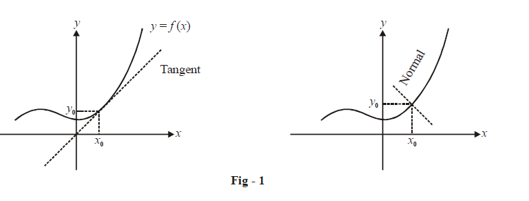
The slope of the tangent at \(x = {x_0}\) would be the value of \(\begin{align}\frac{{dy}}{{dx}}\end{align}\) evaluated at \(x_0:\)
Slope of tangent \(\begin{align}{\left. {\left( {{\rm{at\, }}x = {x_0}} \right){m_T} = \frac{{dy}}{{dx}}} \right|_{x\, = \,{x_0}}}\end{align}\)
Therefore the slope of the normal at \({x_0}\) is:
Slope of normal \(\begin{align}{\left. {\left( {{\rm{at\, }}x = {x_0}} \right){m_N} = \frac{{ - 1}}{{dy/dx}}} \right|_{x = {x_0}}}{\left. { = \frac{{ - dx}}{{dy}}} \right|_{x = {x_0}}}\end{align}\)
Now, since the tangent and normal will pass through the point \(\left( {{x_0},{y_0}} \right)\) and their slopes are known,their equations can be written in a straight forward manner (using the equation of a line passing through a given point with a given slope):
\[\begin{align}\fbox{\(\begin{matrix} \text{Tangent} & : & y-{{y}_{0}} & = & {{m}_{T}}\left( x-{{x}_{0}} \right) & {} & {} \\ \text{Normal} & : & y-{{y}_{0}} & = & {{m}_{N}}\left( x-{{x}_{0}} \right) & = &\begin{align} \frac{-1}{{{m}_{T}}}\end{align}\left( x-{{x}_{0}} \right) \\ \end{matrix}\)}\end{align}\]
For example, suppose that we have to write down the equations of the tangent and normal to \(y=x^{2}\;\text{at}\; x=1:\)
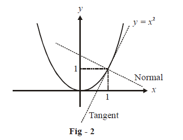
\[\begin{align}{m_T}&={\left. {\frac{{dy}}{{dx}}} \right|_{x = 1}}{\left. { = 2x} \right|_{x = 1}} = 2\\
{m_N}& = \frac{{ - 1}}{{{m_T}}} = \frac{{ - 1}}{2} \end{align}\]
\(\begin{align} & \mathbf{Equation}\text{ }\mathbf{of}\text{ }\mathbf{tangent}:~y-1=2\left( x-1 \right) \\\\
& \qquad \qquad \qquad \qquad\qquad\; \Rightarrow\quad 2x-y-1=0 \\ & \mathbf{Equation}\text{ }\mathbf{of}\text{ }\mathbf{normal}:y-1=\frac{-1}{2}\left( x-1 \right)~ \\ \\ & \qquad \qquad \qquad \qquad\qquad \Rightarrow \quad x+2y-3=0 \end{align}\)
As another example, consider the tangent and normal to \(xy=\text{ }1\text{ }at\;x=\text{ }2:\)
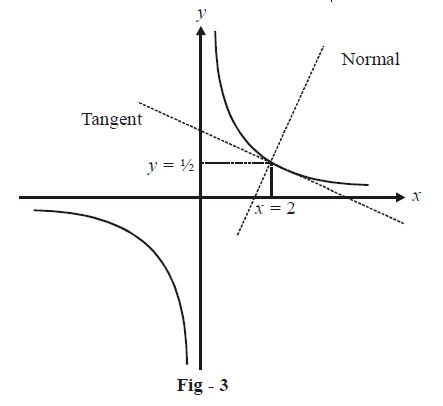
\[\begin{align}{m_T} &={\left. { \frac{{dy}}{{dx}}} \right|_{x = 2}}{\left. { = \frac{{ - 1}}{{{x^2}}}} \right|_{x = 2}} = \frac{{ - 1}}{4}\\{m_N} &= \frac{{ - 1}}{{{m_T}}} = 4\end{align}\]
\(\begin{align}& \mathbf{Equation}\text{ }\mathbf{of}\text{ }\mathbf{tangent}:~y-\frac{1}{2}=\frac{-1}{4}\left( x-2 \right) \\\\ & \qquad \qquad \qquad \qquad\quad\quad\;\; \Rightarrow\quad \text{ }\!\!~\!\!\text{ }x+4y-4=0 \\\\ & \mathbf{Equation}\text{ }\mathbf{of}\text{ }\mathbf{normal}:y-\frac{1}{2}=4\left( x-2 \right) \\ \\& \qquad \qquad \qquad \qquad\qquad\Rightarrow \quad \text{ }\!\!~\!\!\text{ }4x-y-\frac{15}{2}=0 \end{align}\)
As a final example, we are now required to find the angle of intersection between the curves \(y = {x^2}\) and \(\begin{align}y = \frac{1}{x}\end{align}:\)
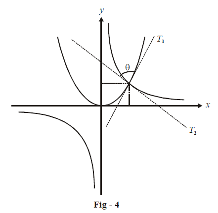
By the angle of intersection between two curves we mean the angle of intersection between the respective tangents to the two curves at their point of intersection, as depicted in Fig.- 4. This angle can be easily evaluated by first finding out the point of intersection of the two curves and then finding out the slopes of the tangents \({{T}_{1}}~\text{ }~and~{{T}_{2}}~\) at this point; for the curves given here, the point of intersection is (1, 1) (verify):
\[\begin{align}{m_{{T_1}}}&={\left. { \frac{{dy}}{{dx}}} \right|_{x = 1}}{\left. { = 2x} \right|_{x = 1}} = 2\\\\
{m_{{T_2}}} &= {\left. {\frac{{dy}}{{dx}}} \right|_{x = 1}}{\left. { = \frac{{ - 1}}{{{x^2}}}} \right|_{x = 1}} = - 1\\\\\Rightarrow \qquad \theta &= \left| {{{\tan }^{ - 1}}\left( {\frac{{{m_{{T_1}}} - {m_{{T_2}}}}}{{1 + {m_{{T_1}}}{m_{T_2}}}}} \right)} \right| = \left| {{{\tan }^{ - 1}}\left( {\frac{3}{{ - 1}}} \right)} \right| = {\tan ^{ - 1}}3\end{align}\]
- Live one on one classroom and doubt clearing
- Practice worksheets in and after class for conceptual clarity
- Personalized curriculum to keep up with school