Visualizing Functions Through Graphs

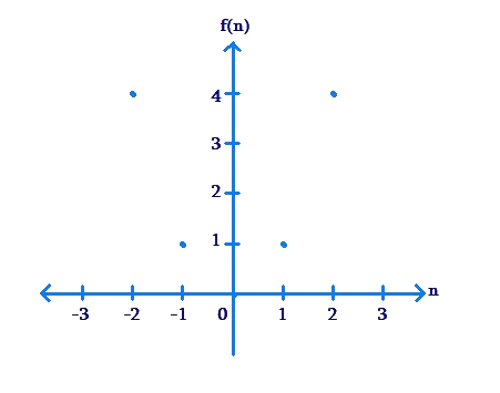
A very powerful way to visualize a function is by graphing it. Let us first consider a very simple example of graphing a function. Suppose that n is an integer in the set {–2, –1,0, 1, 2}. The function f is defined as follows:

\[f\left( n \right) = {n^2}\]

Let us graph this function. On the coordinate axes, we use the horizontal axis for n, and the vertical axis for \(f\left( n \right)\). Note that

\[\begin{array}{l}f\left( { - 2} \right) =4,\,\,\,f\left( { - 1} \right) = 1,\,\,\,f\left( 0 \right) = 0\\f\left( 1 \right) = 1,\,\,\,f\left( 2\right) = 4\end{array}\]

The graph of f is plotted below. Basically, we have plotted the points \(\left({n,f\left( n \right)} \right)\) for all the possible values of n in this case:

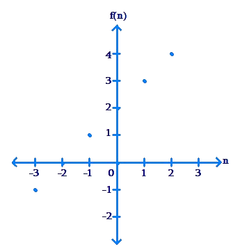
Example 1: n is an integer in the set {–3, –2, –1, 0, 1, 2}. The function f is defined as follows:

\[f\left( n \right) = n + 2\]

Plot the graph of f.

Solution: The graph is plotted below.Verify that all the points on the graph are correct:

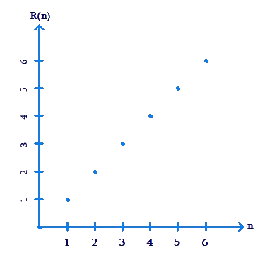
Example 2: In a very slow cricket test match, a team scores 1 run per over for the first six overs. The total score R of the team is a function of the number of overs that have been bowled, n. Plot \(R\left(n \right)\) for the first six overs.

Solution: We note the following:

\[\begin{array}{l}R\left( 1 \right) = 1,\,\,\,R\left( 2\right) = 2,\,\,\,R\left( 3 \right) = 3\\R\left( 4 \right) = 4,\,\,\,R\left( 5\right) = 5,\,\,\,R\left( 6 \right) = 6\end{array}\]

The plot \(R\left( n \right)\) will be as follows:

The function plots discussed till now have been discrete plots: the input variable takes on discrete values.For example, in the last example, n takes values from the discrete set {1, 2, 3, 4, 5, 6}.

What if the input variable takes on a continuous range of values? Consider the function \(f\left( x \right) = x + 2\), where x can take on any real value in the continuous set \(\left[ { - 1,2} \right]\). Observe that the dependence of \(f\left( x \right)\) on x is linear in nature. Thus, the graph of \(f\left(x \right)\) will be a straight line, limited to the input interval \(\left[ { - 1,2} \right]\):

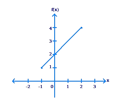
The graph is continuous, not discrete, because the input variable x takes on a continuous range of values, rather than values from a discrete set. Observe that the set of all output values is the continuous set [1, 4].

Example 3: Plot the graph of \(f\left( x \right) = 2x + 1\),if x lies in the set \(\left[ { -\frac{3}{2},\frac{5}{2}} \right]\).

Solution: Once again, \(f\left( x \right)\) is a linear function of x,and hence the graph will be a straight line limited by the input interval:

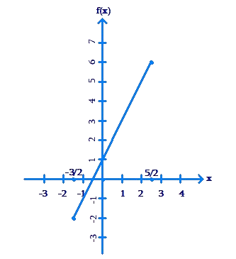
The set of all output values is the continuous set \(\left[ { - 2,6} \right]\).

Example 4: The plot of a function f is shown below.

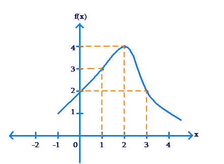
Find the value of \(f\left( 1 \right),\,f\left( 2 \right),\,f\left( 3\right)\).

Solution: The point on the curve having an x-coordinate of 1 is \(\left( {1,3}\right)\). Thus, \(f\left( 1 \right) = 3\).Similarly, we note that \(f\left( 2 \right) = 4\) and \(f\left( 3 \right) = 2\).

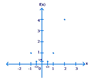
Example 5: Plot the graph of the function \(f\left( x\right) = {x^2}\) if x lies in the interval \(\left[ { - 1,2} \right]\).

Solution: We note that the input set is a continuous rather than a discrete set. How do we plot the graph of the function in this case? We obviously cannot plot points corresponding to all input values(since the set of input values is infinite).

We proceed as follows. First, we determine a few points which will lie on the curve of the function’s graph:

x	\( - 1\)	\( - \frac{1}{2}\)	0	\(\frac{1}{2}\)	1	2
\(f\left( x \right)\)	1	\(\frac{1}{4}\)	0	\(\frac{1}{4}\)	1	4
Point	\(\left( { - 1,1} \right)\)	\(\left( { - \frac{1}{2},\frac{1}{4}} \right)\)	\(\left( {0,0} \right)\)	\(\left( {\frac{1}{2},\frac{1}{4}} \right)\)	\(\left( {1,1} \right)\)	\[\left( {2,4} \right)\]

Next, we plot these points on a pair of axes:

Finally, since the graph for the function should be continuous rather than discrete (because the input set is continuous), we draw a curve passing through these points, as smoothly as we can:

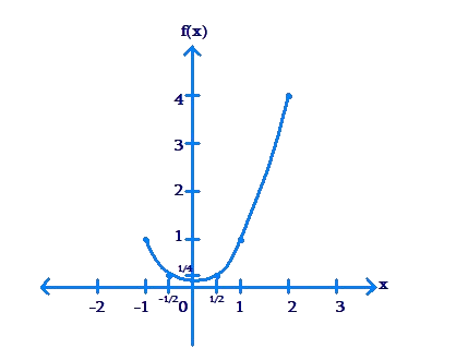
We can then claim that this figure above is the graph of the function.There is an implicit assumption in what we have done: we have assumed that the graph will be a smooth curve, rather than some abrupt or wiggly or other shape. This assumption works in this particular case because the function is a polynomial function.All polynomial functions have smooth curves. We will at a later point discuss scenarios where the curves are not smooth.

Example 6: Plot the graph of the function \(f\left( x\right) = {x^3}\) if x lies in the interval \(\left[ { - \frac{3}{2},1} \right]\).

Solution: Once again, we first determine a few points which will lie on the graph:

x	\( - \frac{3}{2}\)	\( - 1\)	0	\(\frac{1}{2}\)	1
\(f\left( x \right)\)	\( - \frac{{27}}{8}\)	\( - 1\)	0	\(\frac{1}{8}\)	1
Point	\(\left( { - \frac{3}{2}, - \frac{{27}}{8}} \right)\)	\(\left( {1, - 1} \right)\)	\(\left( {0,0} \right)\)	\(\left( {\frac{1}{2},\frac{1}{8}} \right)\)	\(\left( {1,1} \right)\)

Next, we plot these points on a pair of axes. Since \(f\left( x \right) = {x^3}\)is a polynomial function, we make use of the fact that it’s curve will be a smooth curve without abrupt jumps, and so we draw a smooth curve passing through the points we have plotted, which we claim to be the graph of the function:

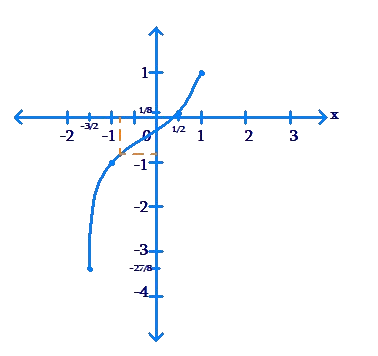
You may verify this claim as follows.Take an x value which is not in the table above. From the graph, read off the corresponding value of \(f\left( x \right)\). Next verify from\(f\left( x \right) = {x^3}\)  whether this value from the graph is the same as (near to) the value calculated algebraically. For example, for \(x = - \frac{3}{4}\) the value from the graph is \(f\left( x \right) \approx  - 0.4\), while the value calculated algebraically is.

\[f\left( x \right) = {\left( { - \frac{3}{4}}\right)^3} =  - \frac{{27}}{{64}} \approx  - 0.42\]

There will of course be small discrepancies in such comparisons because of the approximate nature of hand plots.

There are a number of graph plotters or graphing tools available online. One great example is Geogebra. It will be a very useful exercise for the student to experiment with such tools by plotting the graphs of arbitrary functions. The plots generated by these tool sare very accurate. Here is how any such tool works.

Suppose that you ask the plotter to plot the graph of  \(f\left( x \right) = {x^2}\)  for x lying in the interval \(\left[ { -1,2} \right]\). If you see above, we plotted six sample points or six markers to enable us to draw the plot. However, a computer can do such calculations much faster. The plotter may take 500 input values in this interval, calculate the function output value for each of these input values,and then use 500 markers to draw the plot. The more the markers the plotter uses, the more accurate the final plot will be. Thus, computer based plotters are able to generate very accurate function plots.

Example 7: Plot the graph of the function.

\[f\left( x \right) = \frac{2}{{1 +{x^2}}},\,\,\,x\,\,\,{\rm{in}}\,\,\,\left[ { - 5,5} \right]\]

using all integer input values for markers to guide you.

Solution: We calculate the function value for each of the integers in the set \(\left[ { -5,5} \right]\):

x	\( - 5\)	\( - 4\)	\( - 3\)	\( - 2\)	\( - 1\)	0
\(f\left( x \right)\)	\(\frac{1}{{13}}\)	\(\frac{2}{{17}}\)	\(\frac{1}{5}\)	\(\frac{2}{5}\)	1	2
Point	\(\left( { - 5,\frac{1}{{13}}} \right)\)	\(\left( { - 4,\frac{2}{{17}}} \right)\)	\(\left( { - 3,\frac{1}{5}} \right)\)	\(\left( { - 2,\frac{2}{5}} \right)\)	\(\left( { - 1,1} \right)\)	\(\left( {0,2} \right)\)

 

x	1	2	3	4	5
\[f\left( x \right)\]	1	\[\frac{2}{5}\]	\[\frac{1}{5}\]	\[\frac{2}{{17}}\]	\[\frac{1}{{13}}\]
Point	\[\left( {1,1} \right)\]	\[\left( {2,\frac{2}{5}} \right)\]	\[\left( {3,\frac{1}{5}} \right)\]	\[\left( {4,\frac{2}{{17}}} \right)\]	\[\left( {5,\frac{1}{{13}}} \right)\]

Now, we plot these eleven markers on a pair of axes, and draw a smooth curve through the markers to obtain our plot:

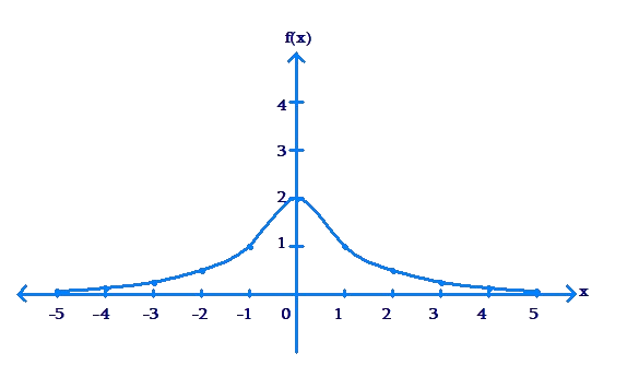
Compare this plot above with the plot of the same function with the input set as the set of Real numbers, using a computer based plotter:

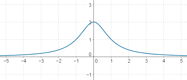
On both sides, the arms of the curve tend to zero level, because as x increases in magnitude, the denominator of the function increases, so the overall function value decreases. When x is very large, the function value is close to zero.